Fourier Transform for Engineers: Practical FFT Applications

Fourier Transform for Engineers: Practical FFT Applications

The Fourier Transform in electronics is one of the most powerful mathematical tools an engineer can have in their toolkit. Whether you are analysing audio signals with an Arduino, debugging noise on a sensor line, or designing digital filters for a DSP project, the Fourier Transform — and its fast computational cousin, the FFT (Fast Fourier Transform) — sits at the heart of the solution. In this guide we break down the theory and then focus on practical, hands-on applications that Indian makers and hobbyists can implement today.

What Is the Fourier Transform?

Joseph Fourier, a 19th-century French mathematician, discovered that any periodic signal — no matter how complex — can be expressed as a sum of simple sine and cosine waves. The Fourier Transform is the mathematical operation that decomposes a signal into its constituent frequencies.

In electronics, every real-world signal is a mix of multiple frequencies. A microphone picking up speech contains frequencies from 300 Hz to 3400 Hz. A motor generates vibration harmonics at multiples of its rotation speed. An ADC reading a sensor line picks up 50 Hz mains hum plus the actual signal. The Fourier Transform lets you see all of these components separately.

The continuous Fourier Transform is defined as:

F(ω) = ∫ f(t) · e^(-jωt) dt

For engineers working with digital systems and microcontrollers, the Discrete Fourier Transform (DFT) is what matters. It operates on sampled data points rather than continuous signals. The DFT of N samples is:

X[k] = Σ x[n] · e^(-j2πkn/N)   for n = 0 to N-1

The key parameters you must understand:

• Sample rate (fs): How many samples per second your ADC takes. An Arduino Uno’s ADC runs at ~9600 samples/sec by default.
• FFT size (N): Number of samples analysed. Common choices: 64, 128, 256, 512, 1024.
• Frequency resolution: fs / N. With fs=9600 and N=256, resolution = 37.5 Hz per bin.
• Nyquist limit: Maximum detectable frequency = fs / 2. Always sample at least twice your highest frequency of interest.

Time Domain vs Frequency Domain

The Fourier Transform is fundamentally a change of perspective. In the time domain, you see amplitude versus time — the waveform as an oscilloscope displays it. In the frequency domain, you see amplitude (or power) versus frequency — the spectrum as a spectrum analyser displays it.

Consider a simple example: You have a 1 kHz square wave. In the time domain it looks like an alternating high-low signal. In the frequency domain, a square wave reveals a rich harmonic content: a fundamental at 1 kHz, then harmonics at 3 kHz, 5 kHz, 7 kHz… falling off as 1/n in amplitude. This is why a square wave through a low-pass filter rounds off — you are removing those high-frequency harmonics.

For Indian makers prototyping on breadboards, this insight is invaluable. That mysterious ringing on your I2C bus? FFT it. That oscillation in your PID control loop? FFT the error signal. The Fourier Transform turns invisible problems visible.

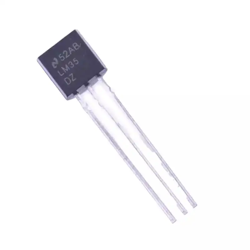
LM35 Temperature Sensors

Ideal for FFT-based signal analysis experiments. Feed the LM35 output into your ADC and use FFT to detect periodic temperature fluctuations or mains noise coupling into your sensor line.

View on Zbotic

FFT Explained: How Computers Compute It Fast

The naive DFT algorithm requires O(N²) operations. For N=1024, that’s over a million multiplications — far too slow for real-time use on a microcontroller. The FFT algorithm, developed by Cooley and Tukey in 1965, reduces this to O(N log N). For N=1024, that’s roughly 10,000 operations — a 100× speedup.

The FFT works by recursively splitting the DFT into smaller DFTs of even-indexed and odd-indexed samples — the Decimation In Time (DIT) approach. The result is a butterfly computation graph that reuses intermediate results. The only constraint: N must be a power of 2 (64, 128, 256, 512, 1024, 2048…).

FFT output interpretation:

• The FFT of N real samples produces N complex numbers (real + imaginary parts).
• Only the first N/2 bins are useful (the rest are mirror images — Hermitian symmetry).
• Magnitude of bin k = sqrt(real[k]² + imag[k]²)
• Power = magnitude²
• Phase = atan2(imag[k], real[k])
• Bin k corresponds to frequency = k × (fs / N)

Windowing: A critical but often missed step. FFT assumes the signal is periodic within the analysis window. If it is not (most real signals), you get spectral leakage — energy from one frequency bin spills into neighbouring bins. Solution: multiply your input samples by a window function before FFT. Common choices: Hann window (good general purpose), Hamming (good for narrowband signals), Blackman (best sidelobe rejection). For most hobbyist audio/sensor work, the Hann window is the right default.

Practical FFT Applications in Electronics

1. Audio Spectrum Analyser

One of the most popular FFT projects in the Indian maker community is an LED spectrum analyser. Sample audio from a microphone module at 8–44 kHz, run FFT on blocks of 256–1024 samples, map the frequency bins to LED bars. Libraries like ArduinoFFT make this straightforward on an Arduino Uno or Nano.

2. Sensor Noise Analysis

Is your DHT11 or LM35 reading noisy? Capture 256 consecutive ADC readings and run FFT. If you see a spike at 50 Hz, your sensor is picking up mains hum — add better decoupling capacitors and shielded wire. If the spike is at some other frequency, it might be motor interference or switching regulator noise from your power supply.

3. Motor and Vibration Monitoring

Attach an accelerometer (ADXL345 or MPU6050) to a motor housing. Sample the vibration at 1 kHz or faster. The FFT spectrum reveals the motor’s rotation frequency and its harmonics. A healthy motor has a clean spectrum with only fundamental and a few harmonics. A bearing with wear develops characteristic fault frequencies. This is industrial-grade predictive maintenance at hobbyist cost.

4. Power Quality Analysis

Sample mains voltage (safely, through a transformer or voltage divider) at ≥10 kHz. FFT shows the fundamental at 50 Hz and harmonics at 100, 150, 200 Hz etc. Total Harmonic Distortion (THD) is directly computable from the FFT output. This is exactly how power quality analysers work commercially.

5. RF Spectrum Sensing

With an RTL-SDR dongle (costs ~₹1500 in India), you can capture 2.4 MHz of RF spectrum at once. Software like GNU Radio or GQRX displays the FFT of the IQ samples in real time. This is how you visualise WiFi channels, FM radio stations, or find interfering transmitters.

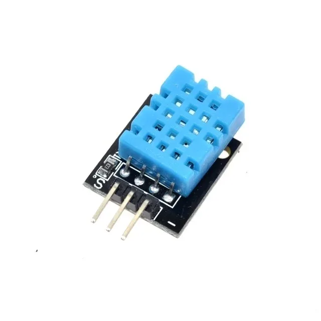
DHT11 Digital Relative Humidity and Temperature Sensor Module

Use the DHT11 with an Arduino to sample temperature data over time and apply FFT to detect periodic environmental patterns or diagnose electrical interference affecting your sensor readings.

View on Zbotic

Running FFT on Arduino and ESP32

The most popular library for FFT on Arduino-compatible boards is ArduinoFFT by Enrique Condes (available in Arduino Library Manager). It supports float and double precision, multiple window functions, and is optimised for AVR and ARM cores.

Here is a minimal working example for an Arduino Uno reading an analog sensor on A0:

#include <arduinoFFT.h>

#define SAMPLES 256
#define SAMPLING_FREQ 2000  // Hz (must be 2x your max freq of interest)

double vReal[SAMPLES];
double vImag[SAMPLES];
arduinoFFT FFT = arduinoFFT();

void setup() {
  Serial.begin(115200);
}

void loop() {
  // Collect samples
  unsigned long samplingPeriodUs = 1000000UL / SAMPLING_FREQ;
  for (int i = 0; i < SAMPLES; i++) {
    unsigned long t = micros();
    vReal[i] = analogRead(A0);
    vImag[i] = 0;
    while (micros() - t < samplingPeriodUs); // wait for next sample
  }

  // Apply window, compute FFT, get magnitudes
  FFT.Windowing(vReal, SAMPLES, FFT_WIN_TYP_HANN, FFT_FORWARD);
  FFT.Compute(vReal, vImag, SAMPLES, FFT_FORWARD);
  FFT.ComplexToMagnitude(vReal, vImag, SAMPLES);

  // Find dominant frequency
  double peak = FFT.MajorPeak(vReal, SAMPLES, SAMPLING_FREQ);
  Serial.print("Dominant frequency: ");
  Serial.print(peak);
  Serial.println(" Hz");

  delay(500);
}

ESP32 advantages for FFT: The ESP32 has a hardware-accelerated FFT in its DSP library (`esp-dsp`). With its 240 MHz dual-core Xtensa processor and 12-bit ADC, the ESP32 can run 1024-point FFT at ~8 kHz update rate — fast enough for serious audio spectrum analysis. The IDF DSP library provides `dsps_fft2r_fc32` for floating-point FFT with SIMD acceleration.

10 x 10 cm Universal PCB Prototype Board Single-Sided 2.54mm Hole Pitch

Build permanent FFT-based spectrum analyser circuits on this sturdy prototype board. Great for moving your breadboard designs to a more reliable form factor.

View on Zbotic

Using FFT for Filter Design

One of the most direct engineering uses of the FFT is designing and verifying digital filters. The connection is the Convolution Theorem: convolution in the time domain equals multiplication in the frequency domain. This means:

• To apply a filter: FFT the signal → multiply by the filter’s frequency response → Inverse FFT
• To design a filter: specify the desired frequency response (e.g., pass 0–500 Hz, reject above) → Inverse FFT to get the filter coefficients (FIR filter taps)

For simple low-pass filtering on a microcontroller, the IIR (recursive) approach is more efficient than FFT-based convolution. But for batch processing of sensor data on a PC, FFT-based filtering (overlap-add or overlap-save method) is the standard approach.

Practical filter design workflow:

1. Capture raw signal and run FFT to understand the noise spectrum
2. Identify the cutoff frequency — where signal ends and noise begins
3. Design filter (Python scipy.signal or MATLAB) with appropriate roll-off
4. Implement as IIR biquad on microcontroller using the filter coefficients
5. Verify by FFT-ing the filtered output

Python example for quick FFT-based analysis (run on your PC with data from Arduino):

import numpy as np
import matplotlib.pyplot as plt

fs = 2000  # sample rate Hz
data = np.loadtxt('sensor_data.csv')  # your Arduino samples

N = len(data)
freqs = np.fft.rfftfreq(N, d=1/fs)
spectrum = np.abs(np.fft.rfft(data * np.hanning(N)))

plt.plot(freqs, 20*np.log10(spectrum + 1e-10))
plt.xlabel('Frequency (Hz)')
plt.ylabel('Magnitude (dB)')
plt.title('Signal Spectrum')
plt.grid(True)
plt.show()

Tools and Hardware for FFT Projects

Building FFT projects requires good hardware fundamentals: clean power, properly decoupled circuits, and appropriate signal conditioning. Here are the essentials:

Decoupling capacitors: Place 100nF ceramic capacitors between VCC and GND at every IC. They filter out high-frequency switching noise that would corrupt your ADC samples and appear as false peaks in your FFT spectrum.

Anti-aliasing filter: Always add a simple RC low-pass filter before your ADC input. Cutoff at fs/2. Without it, frequencies above Nyquist fold back and appear as phantom signals in your spectrum — a phenomenon called aliasing. For fs=2000 Hz, add a 3.3 kΩ resistor and 100nF capacitor (cutoff ~480 Hz).

Stable power supply: FFT projects are sensitive to power supply ripple. Use a regulated 12V SMPS or a proper bench supply rather than a cheap phone charger.

0.1µF 50V Capacitor (Pack of 50)

Essential 100nF decoupling and anti-aliasing capacitors for clean ADC readings in FFT projects. Pack of 50 ensures you have plenty for all your sensor circuits.

View on Zbotic

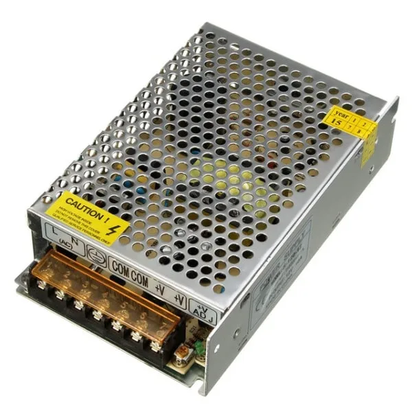
12V 10A SMPS – 120W – DC Metal Power Supply

A stable, regulated 12V power supply is essential for FFT projects where power supply noise corrupts your measurements. Metal enclosure provides EMI shielding.

View on Zbotic

Frequently Asked Questions

What is the difference between DFT and FFT?

DFT (Discrete Fourier Transform) and FFT (Fast Fourier Transform) produce identical results. The FFT is simply a computationally efficient algorithm to compute the DFT. The FFT requires N to be a power of 2 and runs in O(N log N) operations instead of O(N²) for the naive DFT.

What sample rate should I use on Arduino for audio FFT?

Arduino Uno’s default analogRead takes about 104 µs, giving ~9600 samples/sec maximum. To get cleaner timing, use the ADC’s free-running mode which can reach up to 76.9 kSPS (at reduced resolution). For audio work, 8000–9600 Hz sample rate gives frequency coverage up to 4–4800 Hz — sufficient for voice and basic audio analysis.

Why does my FFT show a large spike at 0 Hz (DC)?

A large DC component (bin 0) usually means your signal has a non-zero average value. Subtract the mean of your samples before computing the FFT: vReal[i] -= average;. This removes the DC offset and makes the AC components easier to see.

What is spectral leakage and how do I fix it?

Spectral leakage happens when the frequency you are analysing does not fall exactly on an FFT bin boundary. The energy “leaks” into adjacent bins, smearing the peak. Fix it by applying a window function (Hann, Hamming, Blackman) to your samples before FFT. This trades some frequency resolution for much better sidelobe rejection.

Can I use FFT for real-time processing on ESP32?

Yes. The ESP32’s esp-dsp library includes hardware-accelerated FFT routines that can process 512-point FFT in under 1 ms. Paired with the ESP32’s I2S peripheral for high-quality audio sampling, you can build real-time spectrum analysers, voice-activated devices, and audio effects processors running entirely on the microcontroller.