
A sensor fresh out of the packet rarely gives perfect readings. The raw output deviates from the true physical value due to manufacturing tolerances, aging, temperature drift, and non-linear response curves. Calibration is the process of characterising and correcting these errors so your measurements are trustworthy. Whether you are building a precision weighing scale, a gas detector, or a temperature logger, understanding offset, gain, and linearization calibration will elevate your projects from prototype to professional instrument.
Why Calibration Matters
Consider an LM35 temperature sensor. Its ideal sensitivity is 10 mV/°C. But after 1,000 hours of operation, a specific unit might output 10.2 mV/°C with a 2 mV zero-offset. Without calibration, a 25 °C room reads as 25.4 °C — acceptable for room comfort sensing, but disastrous for pharmaceutical cold-chain monitoring where ±0.5 °C matters. Similarly, a load cell on a postal scale might read 1,015 g for a 1,000 g reference weight. A 1.5% gain error translates to ₹375 error on every 25 kg parcel — a commercial liability.
Calibration does not make a bad sensor good. It characterises the relationship between sensor output and the true physical quantity so you can apply a mathematical correction. Every precision instrument — from laboratory balances to engine management sensors — is calibrated at the factory and recalibrated periodically in the field.
Types of Sensor Error
Before applying corrections, you need to understand what kind of error is present:
- Offset error (zero error): The sensor reads a non-zero value when the input is zero. Example: a pressure sensor showing 12 Pa when exposed to atmospheric reference pressure.
- Gain error (span error, sensitivity error): The sensor’s slope is wrong — it under- or over-reports by a consistent percentage across the range. Example: a load cell outputting 0.97 mV/V instead of 1.00 mV/V.
- Non-linearity: The response curve bends — the percentage error varies with the input level. Example: MQ gas sensors, thermistors, and turbine flow meters all exhibit non-linear curves.
- Temperature drift: Offset and gain both shift with temperature. Example: metal-foil strain gauges drift ~0.01%/°C in gain.
- Hysteresis: The reading differs depending on whether you are approaching from below or above. Common in magnetic sensors and some pressure sensors.
- Repeatability noise: Random scatter around the true value. Reduced by averaging, not by calibration constants.
Offset Calibration
Offset calibration is the simplest correction: measure the sensor output at a known-zero input, then subtract that reading from all subsequent measurements.
Mathematical Model
corrected_value = raw_value - offset
Procedure
- Establish a true-zero condition (e.g., zero weight on scale, 0 Pa differential pressure, 0 °C reference for zero-based sensors).
- Take 50–100 readings at that condition; compute the mean.
- Store the mean as your
offsetconstant. - Subtract it from every future reading.
Arduino Example — Zeroing an ACS712 Current Sensor
const int ACS_PIN = A0;
float acs_offset = 0.0;

void calibrate_zero() {
  long sum = 0;
  for (int i = 0; i < 100; i++) {
    sum += analogRead(ACS_PIN);
    delay(5);
  }
  acs_offset = sum / 100.0; // ADC counts at true zero current
}

float read_current_A() {
  int raw = analogRead(ACS_PIN);
  float voltage = (raw - acs_offset) * (5.0 / 1023.0);
  return voltage / 0.100; // 100 mV/A for ACS712-20A variant
}
Run calibrate_zero() once at startup with no load connected. Every subsequent read_current_A() call will be offset-corrected.
Gain Calibration
Gain (or span) calibration corrects the slope. After offset correction, the sensor output is proportional to the true value but by a slightly wrong factor. You correct it by dividing by (or multiplying by) a gain constant derived from a known reference.
Mathematical Model
calibration_factor = known_reference / sensor_reading_at_reference
corrected_value = raw_reading * calibration_factor
Procedure
- Apply a known, accurate reference stimulus at the high end of your working range (e.g., a calibrated 1 kg mass on a scale).
- Average 50–100 readings to get a stable sensor output.
- Divide the known reference value by the sensor output — that ratio is your gain correction factor.
- Multiply every future reading by this factor.
Arduino Example — HX711 Load Cell Gain Calibration
#include <HX711.h>
HX711 scale;
const float KNOWN_MASS_g = 500.0; // use a calibrated 500g weight

void calibrate_gain() {
  long raw_sum = 0;
  for (int i = 0; i < 50; i++) {
    raw_sum += scale.read();
  }
  float raw_avg = raw_sum / 50.0;
  float calibration_factor = KNOWN_MASS_g / raw_avg;
  EEPROM.put(0, calibration_factor); // store for next power-on
  Serial.print("Calibration factor: ");
  Serial.println(calibration_factor, 6);
}
Two-Point Calibration (Offset + Gain Together)
A two-point calibration corrects both offset and gain simultaneously by measuring at two known reference points: one near zero and one near full-scale. This is the most commonly used calibration in practice because it captures both systematic errors in one procedure.
Mathematical Model
Given two reference points (x1, y1) and (x2, y2) where x is the true value and y is the raw sensor reading:
gain = (x2 - x1) / (y2 - y1)
offset = x1 - gain * y1
corrected = gain * raw + offset
Example — DS18B20 Temperature Sensor Two-Point Calibration
// Reference points measured with certified thermometer:
// At 0°C ice bath  → sensor reads -0.25°C  (y1=-0.25, x1=0)
// At 100°C boiling → sensor reads 99.50°C  (y2=99.5, x2=100)

const float x1 = 0.0, y1 = -0.25;
const float x2 = 100.0, y2 = 99.5;
const float gain = (x2 - x1) / (y2 - y1); // 1.00754...
const float offset = x1 - gain * y1;       // 0.25189...

float calibrated_temp(float raw_temp) {
  return gain * raw_temp + offset;
}
This corrects the DS18B20’s typical ±0.5 °C tolerance to within ±0.1 °C for the 0–100 °C range — a significant improvement for a sensor that costs under ₹50.
Linearization Techniques
Some sensors have fundamentally non-linear response curves. Two-point calibration only helps if the curve is straight. For curved responses, you need linearization.
1. Polynomial Fitting (Curve Fitting)
Measure the sensor output at many known reference points across the full range (10, 20, or more points). Fit a polynomial to the data using least-squares regression. A 2nd- or 3rd-degree polynomial usually captures most sensor non-linearity.
// Thermistor linearization example (3rd-degree polynomial)
// Coefficients obtained from curve fitting tool:
const float A = -0.000231;
const float B = 0.05412;
const float C = -4.328;
const float D = 145.7;

float linearize_thermistor(float adc_raw) {
  return A*pow(adc_raw,3) + B*pow(adc_raw,2) + C*adc_raw + D;
}
Python’s numpy.polyfit() and scipy.curve_fit() make it easy to compute coefficients from your measured calibration data. Paste the coefficients as constants in your Arduino sketch.
2. Look-Up Table (LUT) with Interpolation
For microcontrollers short on floating-point math resources, a look-up table is highly efficient. Store pairs of (raw_value, corrected_value) in a PROGMEM array. At runtime, find the two nearest entries and interpolate linearly between them.
// MQ-135 CO2 LUT (raw ADC → ppm CO2, 16 calibration points)
const int LUT_SIZE = 16;
const int raw_table[LUT_SIZE]  PROGMEM = {100,150,200,250,300,350,400,450,500,550,600,650,700,750,800,850};
const int ppm_table[LUT_SIZE]  PROGMEM = {400,450,520,620,760,930,1120,1350,1620,1940,2320,2760,3280,3900,4630,5500};

float lut_lookup(int raw) {
  if (raw <= pgm_read_word(&raw_table[0])) return pgm_read_word(&ppm_table[0]);
  for (int i = 1; i < LUT_SIZE; i++) {
    int r0 = pgm_read_word(&raw_table[i-1]);
    int r1 = pgm_read_word(&raw_table[i]);
    if (raw <= r1) {
      float t = (float)(raw - r0) / (r1 - r0);
      return pgm_read_word(&ppm_table[i-1]) + t * (pgm_read_word(&ppm_table[i]) - pgm_read_word(&ppm_table[i-1]));
    }
  }
  return pgm_read_word(&ppm_table[LUT_SIZE-1]);
}
3. Steinhart-Hart Equation for NTC Thermistors
NTC thermistors have a very specific non-linear resistance-to-temperature curve that the Steinhart-Hart equation models with three calibration constants (A, B, C):
// 1/T = A + B*ln(R) + C*(ln(R))^3
// Measure R at 3 known temperatures to solve for A, B, C
const float SH_A = 1.009249522e-3;
const float SH_B = 2.378405444e-4;
const float SH_C = 2.019202697e-7;

float thermistor_temp_C(float adc_raw, float R_fixed, float Vcc) {
  float Vout = adc_raw * (Vcc / 1023.0);
  float R_thermistor = R_fixed * Vout / (Vcc - Vout);
  float lnR = log(R_thermistor);
  float T_kelvin = 1.0 / (SH_A + SH_B*lnR + SH_C*lnR*lnR*lnR);
  return T_kelvin - 273.15;
}
Temperature Compensation
Many sensors drift when ambient temperature changes — even sensors that do not measure temperature. Strain gauges, gas sensors, pressure sensors, and load cells all exhibit temperature coefficients. The fix is to measure ambient temperature alongside your primary measurement and apply a correction model.
Simple Linear Temperature Compensation
// Calibrate at two temperatures: T_ref (25°C) and T_hot (50°C)
// Measure offset drift: d_offset_per_C = (offset_hot - offset_ref) / (50 - 25)
// Measure gain drift:   d_gain_per_C   = (gain_hot - gain_ref)   / (50 - 25)

float temperature_compensate(float raw, float ambient_C) {
  float ref_temp = 25.0;
  float adj_offset = offset_ref + d_offset_per_C * (ambient_C - ref_temp);
  float adj_gain   = gain_ref   + d_gain_per_C   * (ambient_C - ref_temp);
  return adj_gain * raw + adj_offset;
}
For temperature-critical applications (lab instruments, food safety sensors), always co-locate a calibrated temperature sensor (DS18B20 or DHT20) alongside your primary sensor and apply compensation in firmware.
Storing Calibration Constants in EEPROM
Calibration constants computed at startup (or entered by the user) must survive power cycling. The Arduino’s built-in EEPROM (1 KB on Uno, 4 KB on Mega) is ideal for this. For ESP32, use the Preferences library; for Raspberry Pi, write constants to a file in /boot or /etc.
#include <EEPROM.h>

struct CalibData {
  float gain;
  float offset;
  uint32_t magic; // 0xCAFEBEEF to detect valid data
};

void save_calibration(float g, float o) {
  CalibData cd = {g, o, 0xCAFEBEEF};
  EEPROM.put(0, cd);
}

bool load_calibration(float &g, float &o) {
  CalibData cd;
  EEPROM.get(0, cd);
  if (cd.magic == 0xCAFEBEEF) {
    g = cd.gain; o = cd.offset;
    return true;
  }
  // No valid data — use defaults
  g = 1.0; o = 0.0;
  return false;
}
Practical Examples by Sensor Type
LM35 Temperature Sensor — Offset + Gain
The LM35 outputs 10 mV/°C with a typical accuracy of ±0.5 °C. For a two-point calibration, dip it in ice-water slurry (0 °C) and boiling water (100 °C at sea level, 98.8 °C in Pune at 560 m altitude). Apply the two-point formula above. Store the gain and offset in EEPROM for a precision thermometer that outperforms its datasheet spec.
DHT11 / DHT20 Humidity — Offset Only
DHT sensors have fixed ±5% RH accuracy that you cannot improve without a humidity reference chamber. However, you can apply a constant offset if you have a reference hygrometer: if DHT reads 52% and reference reads 55%, add +3% offset. The gain of DHT sensors is generally accurate enough that further correction is rarely needed for hobby use.
BMP280 Barometric Pressure — Sea-Level Conversion
BMP280 measures absolute pressure (hPa). To compare readings from different altitudes (weather station use), convert to sea-level pressure using the barometric formula. This is a form of offset calibration where the offset depends on altitude — itself computed from the sensor’s temperature reading. The BMP280 library handles this with seaLevelForAltitude(altitude_m, pressure_hPa).
Load Cells (HX711) — Tare + Span
Load cells are a textbook two-point calibration: tare (zero) with empty scale, then span (gain) with a known weight. The HX711 library’s set_scale() and tare() functions implement this directly. For multi-cell installations (4 cells in a platform scale), average the outputs and apply a single combined calibration factor.
ACS712 Current Sensor — Zero + Sensitivity
At zero current, ACS712 outputs VCC/2 (nominally 2.5 V). Measure the actual voltage at zero current (it may be 2.48 V or 2.52 V) — that is your offset. The sensitivity (mV/A) is specified per variant: 185 mV/A for 5A, 100 mV/A for 20A, 66 mV/A for 30A. To refine sensitivity, pass a known current (use a calibrated ammeter in series) and back-calculate the actual mV/A.
MQ Gas Sensors — Load Resistance Tuning + LUT
MQ sensors require warm-up (24–48 hours) before calibration. Their Rs/R0 ratio is plotted on a log-log curve in the datasheet. Measure Rs at clean air (known baseline), set R0, then use the datasheet graph data to build a LUT mapping Rs/R0 ratios to gas concentrations. Temperature and humidity compensation coefficients are also provided in MQ datasheets and should be incorporated for accurate ppm readings.
Recommended Products from Zbotic

LM35 Temperature Sensor
Classic 10 mV/°C analog sensor — perfect for practicing offset and gain calibration techniques with a stable reference.

DS18B20 Programmable Resolution Temperature Sensor
Two-point calibration brings DS18B20 accuracy to ±0.1 °C — ideal for precision thermal monitoring applications.
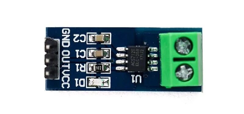
ACS712 5A Current Sensor Module
Hall-effect current sensor that benefits directly from zero-offset calibration at startup for accurate AC/DC power monitoring.
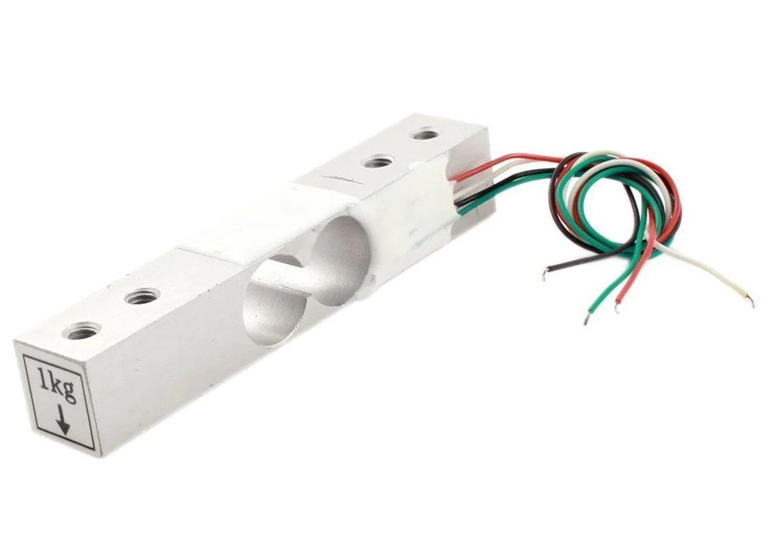
1 Kg Load Cell — Electronic Weighing Scale Sensor
Requires tare + span calibration with HX711 amplifier — the best classroom demonstration of two-point gain calibration.
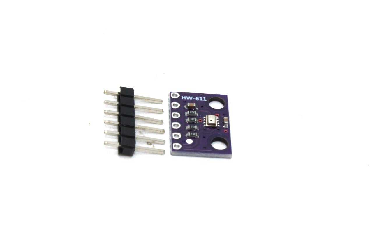
BMP280 Barometric Pressure and Altitude Sensor I2C/SPI
Factory-calibrated pressure sensor with 12 calibration coefficients stored on-chip — a great example of manufacturer-applied polynomial linearization.
Frequently Asked Questions
How often should I recalibrate sensors?
It depends on the application and environment. Industrial standards recalibrate annually or after any significant thermal event. For Arduino hobby projects, recalibrate whenever you notice drift, after reassembling mechanical assemblies (load cells), or after the sensor has been exposed to saturation (MQ gas sensors after being exposed to high gas concentrations). Setting a calibration date in EEPROM and flagging a recalibration reminder after a set number of hours is good practice for critical applications.
Can I calibrate without a traceable reference standard?
You can calibrate against any known reference — it does not have to be NABL/ISO certified for hobby use. Ice-water slurry (0 °C), boiling water (altitude-corrected), certified calibration masses (available from laboratory suppliers), and atmospheric pressure from a trusted weather station API all serve as practical references. For professional instruments, traceability to NABL/NBS standards is required.
What is the difference between accuracy and precision in sensor calibration?
Accuracy is how close to the true value your measurement is. Precision (repeatability) is how consistent your measurements are with each other. Calibration corrects accuracy. Averaging and filtering improve precision. A well-calibrated but noisy sensor has high accuracy and low precision. An uncalibrated but stable sensor has high precision and low accuracy. You need both for a reliable instrument.
My calibration improves accuracy at one temperature but not others. Why?
You performed a single-temperature calibration and ignored temperature coefficient of the sensor. The offset and gain you measured at 25 °C may shift by 2–5% at 45 °C. Implement temperature compensation as described above, or perform your calibration at the actual operating temperature of your final installation.
Does averaging replace calibration?
No. Averaging reduces random noise (improving precision) but cannot remove systematic errors like offset or gain errors, which appear consistently in every reading. You need both calibration (for accuracy) and averaging (for precision). A simple 32-sample moving average combined with two-point calibration gives dramatically better results than either technique alone.
Shop Zbotic’s complete range of sensors and measurement modules — temperature, pressure, current, gas, and more. All products ship with datasheets. Free shipping above ₹999.


Add comment