
Mastering robot arm 6-DOF inverse kinematics with Python and ROS is the gateway to building truly capable robotic manipulators. Whether you are programming a physical servo arm, working with a NEMA17 stepper-driven 6-DOF arm, or using simulation in Gazebo, understanding inverse kinematics (IK) is essential to moving an end-effector to any point in 3D space. This tutorial covers the mathematics, the Python libraries, ROS MoveIt 2 integration, and how to apply everything to real hardware you can buy in India.
What Is Inverse Kinematics and Why Does It Matter?
Inverse Kinematics (IK) answers this question: given a desired position (X, Y, Z) and orientation (roll, pitch, yaw) for the robot arm’s end-effector (the gripper or tool tip), what angles must each of the 6 joints be set to in order to reach that pose?
This is the opposite of Forward Kinematics (FK), which answers: given the joint angles, where is the end-effector? FK is a simple chain of matrix multiplications. IK is mathematically much harder — for a 6-DOF arm the system of equations may have multiple solutions, one solution, or no solution depending on whether the target pose is within the arm’s reachable workspace.
IK is what makes robot arms useful. Instead of manually figuring out “set joint 1 to 45°, joint 2 to -30°…” every time you want to pick up an object, you simply say “move gripper to (x=0.3m, y=0.1m, z=0.2m)” and the IK solver figures out all 6 joint angles automatically.
Forward Kinematics vs Inverse Kinematics
A clear comparison before diving into the math:
| Aspect | Forward Kinematics (FK) | Inverse Kinematics (IK) |
|---|---|---|
| Input | Joint angles (θ1…θ6) | Desired end-effector pose (X,Y,Z,R,P,Y) |
| Output | End-effector pose | Joint angles (θ1…θ6) |
| Solution uniqueness | Always one solution | Zero, one, or infinite solutions |
| Computation | Simple (matrix multiply) | Complex (iterative or analytical) |
| Use case | Visualisation, trajectory checking | Task-space motion planning |
Denavit-Hartenberg Parameters Explained
The Denavit-Hartenberg (DH) convention is the standard way to describe the geometry of a robot arm. Each link/joint transition is described by 4 parameters:
- a (link length): Distance between Z-axes of consecutive joints along the common normal
- d (link offset): Distance along the Z-axis from the common normal of the previous to the current joint
- α (twist angle): Angle between Z-axes around the common normal
- θ (joint angle): The variable — this is what the motor controls
For a 6-DOF arm, you define a 6×4 DH parameter table. Example for a simplified 3-DOF planar arm:
Joint | a    | d   | alpha | theta
  1   | 0    | 0   | 90°   | θ1 (variable)
  2   | L1   | 0   | 0°    | θ2 (variable)
  3   | L2   | 0   | 0°    | θ3 (variable)

Where L1, L2 are link lengths in meters
The DH transformation matrix for each joint converts from one joint frame to the next. Multiplying all 6 transformation matrices gives the full FK solution — the pose of the end-effector relative to the base.
Solving IK in Python with ikpy
ikpy is the most beginner-friendly Python library for robot arm kinematics. Install it:
pip install ikpyDefine your robot arm from a URDF file or manually with DH parameters:
from ikpy.chain import Chain
from ikpy.link import OriginLink, URDFLink
import numpy as np

# Define a 3-link planar arm
arm = Chain(name='robot_arm', links=[
    OriginLink(),
    URDFLink(name="joint1", origin_translation=[0,0,0],
             origin_orientation=[0,0,0],
             rotation=[0,0,1]),  # rotates around Z
    URDFLink(name="joint2", origin_translation=[0.15,0,0],
             origin_orientation=[0,0,0],
             rotation=[0,0,1]),
    URDFLink(name="joint3", origin_translation=[0.12,0,0],
             origin_orientation=[0,0,0],
             rotation=[0,0,1]),
])

# Solve IK for target position
target_position = [0.2, 0.15, 0.0]
joint_angles = arm.inverse_kinematics(target_position)
print("Joint angles (radians):", joint_angles[1:-1])
print("Joint angles (degrees):", np.degrees(joint_angles[1:-1]))
ikpy uses SLSQP numerical optimisation internally. For a 6-DOF arm, load the URDF file directly:
from ikpy.chain import Chain
arm_chain = Chain.from_urdf_file(
    "robot_arm.urdf",
    active_links_mask=[False, True, True, True, True, True, True, False]
)

target_frame = np.eye(4)
target_frame[:3, 3] = [0.3, 0.1, 0.2]  # X, Y, Z in meters

angles = arm_chain.inverse_kinematics_frame(
    target_frame,
    initial_position=[0]*8
)
Numerical IK Methods: Jacobian and CCD
Two main numerical methods for IK:
Jacobian Transpose / Pseudo-Inverse
The Jacobian matrix J maps joint velocity (θ̇) to end-effector velocity (ẋ). To solve IK iteratively:
# Iterative Jacobian IK (simplified)
error = target_pos - current_pos
delta_theta = J.T @ error  # Jacobian transpose method
theta += alpha * delta_theta  # alpha = step size
The Jacobian pseudo-inverse method (J† = J^T(JJ^T)^-1) gives more accurate convergence. Near singularities (when the arm is fully extended or certain joints align), the Jacobian becomes ill-conditioned — use Damped Least Squares (DLS) to avoid numerical blowup.
CCD (Cyclic Coordinate Descent)
CCD is simpler and more robust. Starting from the last joint and working backwards to the base, it rotates each joint to minimise the distance from end-effector to target. One pass through all joints is one iteration. Typically converges in 10–50 iterations. CCD is preferred for real-time IK on microcontrollers because it requires no matrix inversion.
MoveIt 2: IK and Motion Planning in ROS2
MoveIt 2 is the standard motion planning framework in ROS2. It wraps IK solving, collision checking, and trajectory execution into a clean API. Setup process:
- Create a URDF/xacro of your robot arm — define all links, joints, and joint limits
- Run MoveIt Setup Assistant:
ros2 launch moveit_setup_assistant setup_assistant.launch.py— generates the MoveIt configuration package - Launch MoveIt with your robot:
ros2 launch your_arm_moveit_config demo.launch.py - Plan and execute via Python API:
from moveit.python_bindings import MoveItPy

moveit = MoveItPy(node_name="my_arm_controller")
arm = moveit.get_planning_component("arm_group")

# Set target pose
from geometry_msgs.msg import Pose
target = Pose()
target.position.x = 0.3
target.position.y = 0.0
target.position.z = 0.4
target.orientation.w = 1.0

arm.set_pose_goal(target)
plan = arm.plan()
moveit.execute(plan, controllers=[])
MoveIt 2’s default IK plugin is KDL (Kinematics and Dynamics Library). For better performance on 6-DOF arms, use TRAC-IK or BioIK plugins which handle redundant configurations and near-singularity cases much better than KDL.

ACEBOTT ESP32 5-DOF Robot Arm Kit Expansion Pack – QD007
A 5-DOF ESP32 robot arm kit — ideal for learning and applying inverse kinematics algorithms. Start with Python IK and progress to full ROS2 MoveIt 2 integration.
Applying IK to Real Servo/Stepper Arm Hardware
Running IK on a PC/Pi and sending angles to the physical arm:
Servo Arm (SG90/MG90S)
The IK solver outputs angles in radians. Convert to degrees, offset by the servo’s neutral position (typically 90° = straight), and send via PWM:
# On Raspberry Pi with serial to Arduino
import serial, numpy as np
port = serial.Serial('/dev/ttyUSB0', 115200)

def send_angles(joint_angles_rad):
    degrees = np.degrees(joint_angles_rad)
    cmd = ','.join([str(int(a)) for a in degrees]) + 'n'
    port.write(cmd.encode())
Stepper Arm (NEMA17 + A4988)
Stepper arms with position encoders or known step counts are more accurate. Map IK output angles to steps:
STEPS_PER_DEGREE = 3200 / 360  # 3200 steps/rev (1/16 microstepping)
steps = int(angle_degrees * STEPS_PER_DEGREE)
ACEBOTT ESP32 Programmable Robot Arm Kit for Beginners – QD022
A beginner-friendly ESP32 robot arm kit with servo joints — the perfect physical platform to implement and test your Python IK algorithms on real hardware.

42HS48-1204A NEMA17 5.6 kg-cm Stepper Motor with Detachable Cable
The standard actuator for 6-DOF robot arm joints controlled by IK algorithms — delivers precise, repeatable positioning for every joint in your arm build.
Understanding Workspace and Joint Limits
The workspace of a 6-DOF robot arm has two components:
- Reachable workspace: All positions the end-effector can reach with at least one orientation. Shaped like a thick shell around the arm’s base.
- Dexterous workspace: Positions where the end-effector can reach with any orientation. Smaller than reachable workspace, typically a sphere near the arm’s centre of reach.
Joint limits directly constrain the workspace. Always define joint limits in your URDF — IK solvers that ignore limits can command physically impossible poses. Typical SG90-servo arm joint limits:
- Base rotation (J1): -150° to +150° (or limited by cable routing)
- Shoulder (J2): -90° to +90°
- Elbow (J3): -120° to +120°
- Wrist pitch (J4): -90° to +90°
- Wrist roll (J5): -180° to +180°
- Gripper (J6): 0° to 90° (open/close)
Singularities occur when two or more joint axes align, causing the Jacobian to lose rank. At a singularity the arm loses one or more DOF temporarily. The two common singularities for 6-DOF arms are: arm fully extended (shoulder singularity) and wrist joints aligned (wrist singularity). Always add singularity detection in your IK code and handle gracefully.
Project Ideas Using 6-DOF IK
- Pick-and-Place Robot: Use a depth camera to detect object positions. Feed XYZ to IK solver. Arm moves to object, gripper closes, moves to bin, gripper opens. The classic industrial automation task, achievable in India with off-shelf components.
- Drawing Robot: Define a 2D path in tool space. Sample it at 10 mm intervals. Convert each XY point (with fixed Z=0 on the drawing surface) to joint angles via IK. Execute the trajectory. The arm draws the specified shape.
- Teleoperation with 3D Mouse: Map 3D mouse (SpaceMouse) XYZ deltas to IK target position deltas in real time. Operator moves the mouse; robot arm follows in Cartesian space.
- Surgical Training Phantom: Use IK to guide an arm along pre-programmed surgical paths with sub-millimetre accuracy. Vision-based correction loop keeps the path accurate despite mechanical slop.
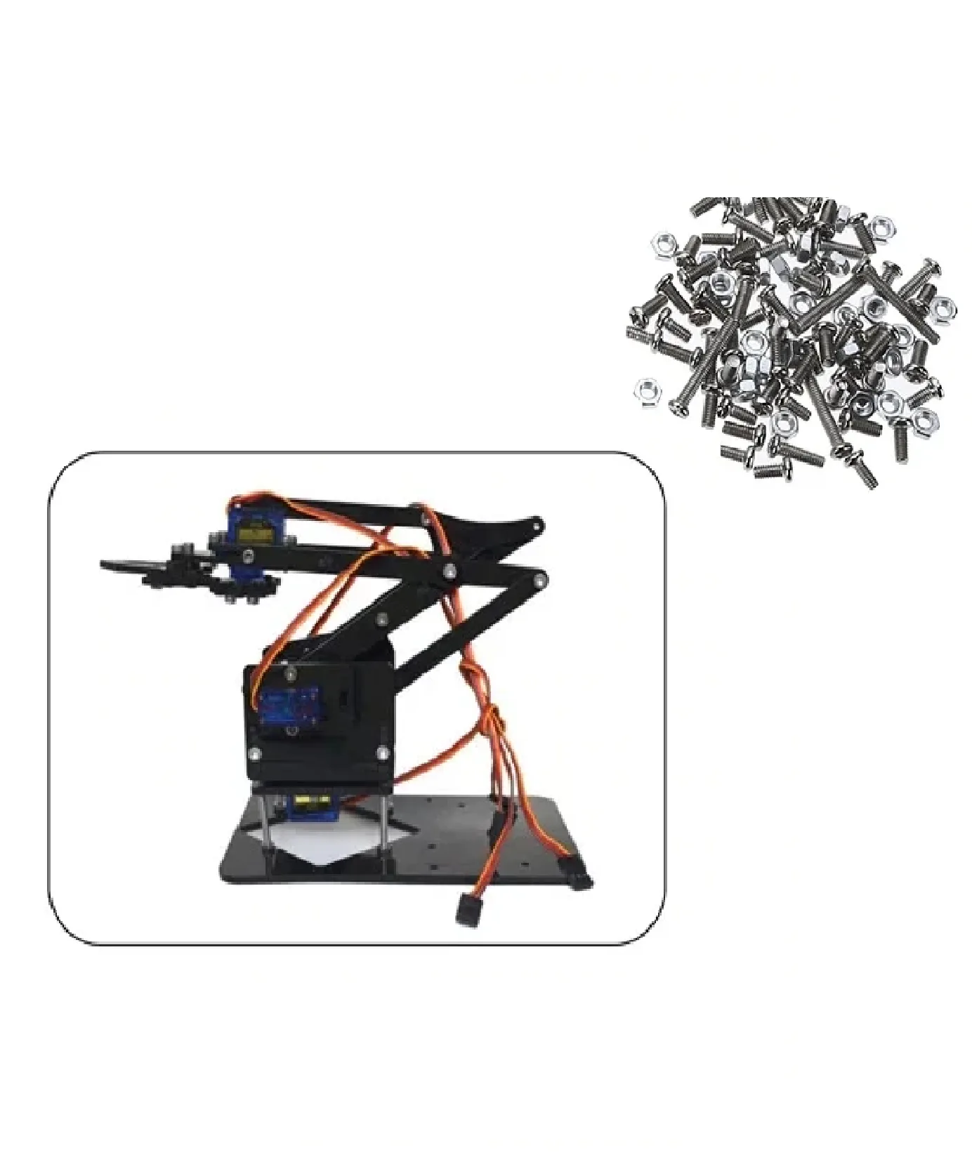
DIY Acrylic Robot Manipulator Mechanical Arm Kit
A complete servo-ready acrylic robot arm — bring your IK code to life on this physical manipulator frame that you can extend, modify, and mount sensors on.
Frequently Asked Questions
What is the difference between 6-DOF and 5-DOF robot arms for IK?
A 6-DOF arm can reach any position in its workspace with any orientation — it has full Cartesian freedom. A 5-DOF arm can reach most positions but has a constrained orientation at those positions. 6-DOF is needed for tasks where the end-effector approach angle matters (e.g., inserting a plug, pouring liquid). 5-DOF is sufficient for most pick-and-place tasks.
Is ikpy or MoveIt better for beginners in India?
Start with ikpy — it is a pure Python library with no ROS dependency, installs in 30 seconds, and you can test IK on your laptop immediately. Once your algorithm is proven, graduate to MoveIt 2 in ROS2 for real robot deployment with collision avoidance and trajectory planning.
Can I run IK in real-time on an Arduino?
Numerical IK (CCD method) can run on a Mega at 10–20 Hz for 3-DOF arms. For 6-DOF, it is better to run IK on a Raspberry Pi or laptop and send precomputed joint angles to the Arduino over serial. The Arduino then handles PWM servo control and safety checks.
What URDF file format does MoveIt 2 need?
MoveIt 2 uses URDF (Unified Robot Description Format) or xacro (XML macro) files. Most robot arm designs on Thingiverse and GitHub include a URDF file. If not, you can create one using Fusion 360’s URDF exporter plugin or the online URDF builder tools.
How accurate are servo-based robot arms with IK in practice?
SG90-based servo arms typically achieve ±5–10 mm end-effector accuracy due to servo resolution (1°), gear backlash, and link flex. NEMA17 stepper arms with 1/16 microstepping achieve ±1–2 mm. For precision pick-and-place, add a vision-based correction loop using a camera and OpenCV to compensate for mechanical error.
Get Your Robot Arm Hardware from Zbotic
From servo arms to NEMA17 stepper assemblies, Zbotic stocks everything you need to build and program a 6-DOF robot arm with IK in India — with fast shipping and expert support.


Add comment