
Resonant Circuit: Series and Parallel LC Resonance Guide
At the heart of radio receivers, signal generators, oscillators, and power converters lies one of electronics’ most elegant phenomena: LC resonance. A resonant circuit — whether series or parallel — is formed by connecting an inductor (L) and a capacitor (C) so that their frequency-dependent reactances cancel each other out at a specific frequency. The result is a circuit that responds dramatically to signals at its resonant frequency while largely ignoring all others. Understanding LC resonance is essential for anyone working with RF electronics, communications, or precision analogue design in India or anywhere in the world.
The Concept of Resonance in LC Circuits
Resonance occurs when the inductive reactance (XL = 2πfL) and capacitive reactance (Xc = 1/2πfC) of the circuit are equal in magnitude. At this specific frequency — the resonant frequency (f₀) — the reactances cancel each other out, leaving only the resistive losses in the circuit.
To understand this intuitively, think of energy sloshing back and forth between the inductor’s magnetic field and the capacitor’s electric field — like a pendulum swinging between kinetic and potential energy. Without losses, this exchange would continue forever at exactly one natural frequency. With losses (resistance in the circuit), the oscillations gradually die out unless maintained by an external signal or active feedback.
Setting XL = Xc to Find Resonant Frequency
2πf₀L = 1/(2πf₀C)
(2πf₀)² = 1/(LC)
f₀ = 1 / (2π√(LC))
This single formula governs both series and parallel LC resonance. It is arguably the most important equation in RF electronics design.
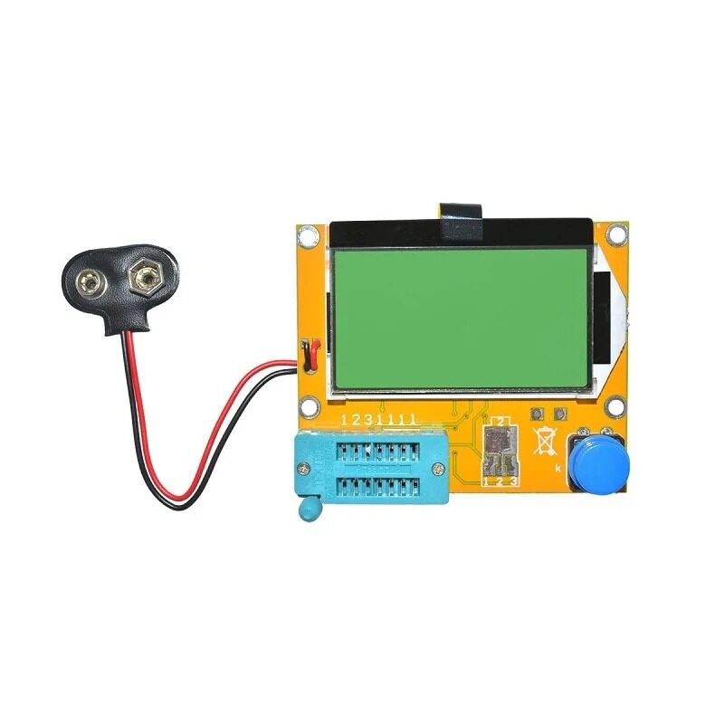
LCR-T4 LCD Graphical Transistor Tester
Accurately measure your inductors and capacitors before building resonant circuits. The LCR-T4 provides L, C, and ESR readings — the exact values you need to predict the resonant frequency accurately.
Series LC Resonance: Theory and Analysis
In a series resonant circuit, the inductor (L), capacitor (C), and a resistance (R — often just the inductor’s winding resistance) are all connected in series with the AC source.
Impedance of a Series RLC Circuit
Z = R + j(XL − Xc) = R + j(ωL − 1/ωC)
At resonance (f = f₀), XL = Xc, so the imaginary parts cancel:
Z_resonance = R (purely resistive, minimum impedance)
Key Characteristics at Series Resonance
- Impedance is minimum and purely resistive (Z = R)
- Current is maximum: I = V_source / R
- Phase angle is zero: Current and source voltage are in phase
- Voltages across L and C can be very large — each can equal Q × V_source! This is called voltage magnification or resonance rise of voltage.
- Power factor = 1 (maximum real power delivered to circuit)
Voltage Magnification at Series Resonance
This is one of the most counter-intuitive aspects of series resonance: the voltage across the individual L or C can be much larger than the source voltage.
V_L = V_C = Q × V_source
For a circuit with Q = 50 and V_source = 5V RMS, the voltage across the capacitor (and across the inductor) would be 50 × 5 = 250V RMS! This is why capacitor voltage ratings in resonant circuits must be derated significantly — a dangerous effect if overlooked.
Frequency Response
The current in a series resonant circuit as a function of frequency is:
I(f) = V / √(R² + (2πfL − 1/(2πfC))²)
This produces a bell-shaped (resonance) curve centred on f₀. The sharpness of this peak is determined by the Q factor.

0.1µF Ceramic Capacitor (Pack of 50)
NP0/C0G type ceramic capacitors are ideal for resonant circuits due to their excellent temperature stability. Their capacitance barely shifts with temperature — keeping your resonant frequency stable even as the circuit heats up.
Parallel LC Resonance (Tank Circuit)
The parallel resonant circuit — often called a tank circuit — connects L and C in parallel. This is the configuration used in oscillators (Colpitts, Hartley), RF amplifier tuned loads, and bandpass filters.
Impedance of a Parallel RLC Circuit
For a parallel LC circuit with a resistance R in parallel:
Y = G + j(Bc − BL) = 1/R + j(ωC − 1/ωL)
Z = 1/Y
At parallel resonance, the susceptances cancel (Bc = BL):
Z_resonance = R (purely resistive, MAXIMUM impedance)
Key Characteristics at Parallel Resonance
- Impedance is maximum and purely resistive (Z = R_parallel)
- Current from the source is minimum — the tank circuit circulates large reactive currents internally
- Circulating current magnification: The current circulating within the L-C loop is Q times the source current — called current magnification
- Phase angle is zero: Source current and voltage are in phase
- Acts as a high-impedance load at resonance — useful as a tuned load for RF amplifiers
Practical Tank Circuit with Winding Resistance
A real inductor has winding resistance r. The resonant frequency of a practical tank circuit (inductor with series resistance r in parallel with ideal C) is:
f₀ = (1/2π) × √(1/LC − r²/L²)
For high-Q inductors (Q > 10), r²/L² << 1/LC and the formula simplifies to the ideal f₀ = 1/(2π√LC) with negligible error.
Dynamic Resistance of the Parallel Tank
At resonance, the parallel tank circuit presents a purely resistive impedance called the dynamic resistance (Rd):
Rd = L / (C × r) = Q × XL = Q² × r
Where r is the inductor’s winding resistance. Higher Q means higher dynamic resistance — the tank circuit presents a very high impedance at resonance, making it excellent as an RF amplifier load that only amplifies signals near f₀.
Q Factor and Bandwidth
The quality factor Q quantifies the selectivity (sharpness) of a resonant circuit. It is defined as:
Q = f₀ / BW = (2π × f₀ × Energy stored) / (Energy dissipated per cycle)
For a series RLC circuit: Q = XL/R = (2πf₀L)/R = 1/(2πf₀CR)
Bandwidth
The bandwidth (BW) of the resonance peak is the range of frequencies between the two −3 dB points (where response drops to 70.7% of peak):
BW = f₀ / Q (Hz)
Example calculations:
- f₀ = 1 MHz, Q = 100 → BW = 10 kHz (very selective, good for single-station radio tuning)
- f₀ = 1 MHz, Q = 10 → BW = 100 kHz (less selective, passes a wider range)
- f₀ = 1 MHz, Q = 5 → BW = 200 kHz (broad — picks up many stations simultaneously)
The Q-Bandwidth Trade-off
High Q = narrow bandwidth = high selectivity = difficult to achieve (requires low-loss components). Low Q = wide bandwidth = easier to build but poor selectivity. The Q factor is ultimately limited by inductor winding resistance. Using high-Q inductors (wound on low-loss ferrite cores or using silver-plated wire) is key to achieving high selectivity in radio tuner circuits.
| Q Factor | BW at 1 MHz | Selectivity | Typical Application |
|---|---|---|---|
| 5–10 | 100–200 kHz | Low | Wideband amplifier loads |
| 20–50 | 20–50 kHz | Moderate | AM radio tuning |
| 100–300 | 3–10 kHz | High | SSB/CW radio filters |
| 1000+ | 1 kHz | Very high | Crystal filters, precision oscillators |
Resonant Frequency Formula and Calculations
Standard Resonant Frequency Formula
f₀ = 1 / (2π√(LC))
Worked Examples
Example 1: Find f₀ for L = 100 µH, C = 100 pF
f₀ = 1 / (2π × √(100×10⁻⁶ × 100×10⁻¹²))
f₀ = 1 / (2π × √(10⁻¹⁴))
f₀ = 1 / (2π × 10⁻⁷)
f₀ = 1.59 MHz — in the AM radio band!
Example 2: Design a tank circuit for 100 MHz FM radio
Choose C = 10 pF (practical minimum for stability)
L = 1 / (4π² × f₀² × C) = 1 / (4π² × (100×10⁶)² × 10×10⁻¹²)
L = 1 / (4π² × 10¹⁶ × 10⁻¹¹)
L = 0.253 µH = 253 nH — about 3 turns of 0.5 mm wire on a 5 mm former
Example 3: Find capacitance for f₀ = 7 MHz (40m amateur band), L = 2.5 µH
C = 1 / (4π² × f₀² × L) = 1 / (4π² × (7×10⁶)² × 2.5×10⁻⁶)
C = 207 pF — easily achievable with standard capacitor values
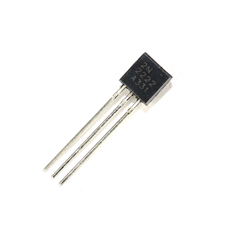
2N2222 NPN Transistor (Pack of 20)
Pair a resonant LC tank circuit with a 2N2222 transistor to build a complete Colpitts or Hartley oscillator. The 2N2222’s high fT makes it suitable for tank circuits up to 30 MHz.
Series vs Parallel Resonance: Key Differences
| Property | Series Resonance | Parallel Resonance |
|---|---|---|
| Impedance at f₀ | Minimum (= R) | Maximum (= Rd) |
| Current at f₀ | Maximum | Minimum (from source) |
| Magnification | Voltage (V_L = V_C = Q×V) | Current (I_L = I_C = Q×I) |
| Phase angle at f₀ | 0° (in phase) | 0° (in phase) |
| Below f₀ | Capacitive (Z rises) | Inductive (Z rises) |
| Above f₀ | Inductive (Z rises) | Capacitive (Z drops) |
| Main applications | Band-pass filters, series traps | Oscillator tanks, tuned RF amps |
Applications of Resonant Circuits
1. Radio Receiver Tuning (India’s Popular Hobbyist Project)
The classic AM radio receiver uses a parallel tank circuit (ferrite rod antenna + variable capacitor) to select a single station from the broadcast band (530–1700 kHz in India). Rotating the variable capacitor tunes the resonant frequency to match the desired station’s carrier frequency. Only that station’s signal sees the high-impedance tank and is amplified; all others are attenuated.
2. Oscillator Tank Circuits
Every LC oscillator — Colpitts, Hartley, Clapp — uses a parallel resonant circuit as its frequency-determining element. The active device (transistor or op-amp) compensates for the tank circuit’s losses (Q degradation from resistive losses) to sustain oscillation at exactly f₀.
3. Impedance Matching Networks
In RF power amplifiers, the output impedance must be transformed from the transistor’s low output impedance (1–5 Ω typical) to the antenna impedance (50 Ω). L-networks, π-networks, and T-networks all use LC resonant circuit principles to accomplish this transformation efficiently.
4. Crystal Filters (Q > 10,000)
A quartz crystal is a mechanical resonator that behaves as an extremely high-Q LC circuit (Q in the range 10,000 to 1,000,000). Crystal filters provide the very narrow bandwidths (300 Hz to 3 kHz) required for SSB and CW radio communications.
5. Induction Heating
Industrial induction heaters and domestic induction cooktops use high-power series resonant circuits operating at 20–100 kHz. At resonance, the high circulating current in the work coil generates intense magnetic flux that inductively heats the cooking vessel or workpiece.
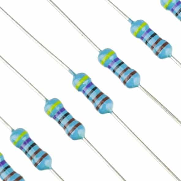
1.5 Ohm 1/4W Metal Film Resistor MFR (Pack of 100)
Use low-value precision resistors to set the Q factor and damping in experimental resonant circuits. Metal film resistors have lower noise and tighter tolerance (±1%) than carbon film — important for accurate resonance measurements.
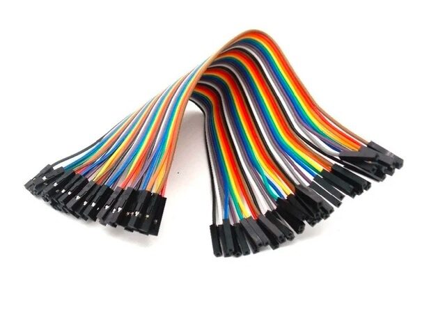
10CM Female To Female Breadboard Jumper Wires 2.54MM – 40Pcs
Connect modules and components when building resonant circuit experiments. F-F jumper wires are perfect for connecting signal generators and oscilloscopes to your breadboard test circuit.
Frequently Asked Questions
What is the resonant frequency of an LC circuit and how is it calculated?
The resonant frequency is the frequency at which inductive reactance equals capacitive reactance (XL = Xc), causing them to cancel. The formula is f₀ = 1/(2π√(LC)), where L is inductance in Henries and C is capacitance in Farads. For example, with L = 100µH and C = 1nF: f₀ = 1/(2π × √(10⁻⁴ × 10⁻⁹)) = 1/(2π × √(10⁻¹³)) = 1/(2π × 3.16×10⁻⁷) ≈ 503 kHz.
What is the difference between series and parallel resonance?
In series resonance, L and C are in series: impedance is minimum at f₀, current from the source is maximum, and voltage magnification occurs across L and C individually. In parallel resonance (tank circuit), L and C are in parallel: impedance is maximum at f₀, current from the source is minimum, and current magnification occurs within the LC loop. Both resonate at the same frequency (f₀ = 1/2π√LC for ideal components), but their impedance behaviour is opposite.
How does Q factor affect the bandwidth of an LC resonant circuit?
The bandwidth (BW) is inversely proportional to Q: BW = f₀/Q. A high-Q circuit (low loss, minimal resistance) has a narrow bandwidth and is very selective — it responds strongly only to frequencies very close to f₀. A low-Q circuit has a wide bandwidth and responds to a broader range of frequencies. For radio receiver design, higher Q means better rejection of adjacent channels. Practical LC circuits achieve Q of 20–200; crystal resonators achieve Q of 10,000 to 1,000,000.
Why is voltage much higher than the source voltage across L and C at series resonance?
At series resonance, the impedance drops to just the small resistance R. With maximum current flowing, the voltage across L is V_L = I × XL and across C is V_C = I × Xc. Since I = V_source/R and XL = Q×R, we get V_L = V_C = Q × V_source. This voltage magnification can be dangerous — in a circuit with Q=100 and a 10V source, individual component voltages reach 1000V. Always check capacitor and inductor voltage ratings when designing series resonant circuits.
What components affect the resonant frequency most in a practical LC circuit?
The resonant frequency depends on L and C values. In practice, stray (parasitic) capacitances from PCB traces, component leads, and transistor output capacitance add to the intended C, shifting f₀ lower than calculated. Stray inductance from component leads adds to the intended L. At high frequencies (>10 MHz), these parasitic effects become significant. Mitigation: measure actual component values (LCR meter), use short leads, keep PCB traces short, and include a small trimmer capacitor for final frequency adjustment.
Start Building LC Resonant Circuits Today
Get capacitors, resistors, transistors, and test equipment from Zbotic — everything you need to build and experiment with series and parallel resonant circuits. Fast shipping across all of India.


Add comment