
Infrared proximity sensors like the Sharp GP2Y series are widely used in robotics, obstacle avoidance, and automation projects — but their output is notoriously non-linear. Unlike ultrasonic sensors that give a direct distance value, IR proximity sensors output a voltage that follows an inverse power-law curve with respect to distance. Without proper IR proximity sensor calibration and an accurate distance vs voltage curve, your robot will misjudge obstacles and your automation logic will trigger at the wrong distances. This tutorial explains how IR sensors work, how to plot and use the distance-voltage curve, and how to implement accurate distance measurement in Arduino.
How IR Proximity Sensors Work
Infrared proximity sensors use the principle of triangulation, not time-of-flight (that is ultrasonic’s domain). The sensor contains an IR LED that emits a continuous beam of infrared light and a Position-Sensitive Detector (PSD) that measures where the reflected IR beam lands on its linear array.
When an object is close to the sensor, the reflected beam hits the PSD at a steep angle — the spot falls far from center. When an object is farther away, the reflected beam arrives at a shallower angle — the spot is closer to center. The PSD outputs a voltage proportional to the spot position, which the sensor’s internal circuit converts to an analog output voltage. This triangulation principle makes the Sharp GP2Y sensors quite immune to the target’s surface color and reflectivity, unlike simpler LED-photodiode proximity sensors.
Common IR proximity sensor models:
| Model | Range | Type | Output |
|---|---|---|---|
| GP2Y0A21YK0F | 10–80 cm | Analog | Most popular, general use |
| GP2Y0A02YK0F | 20–150 cm | Analog | Long range |
| GP2Y0A41SK0F | 4–30 cm | Analog | Short range |
| Simple IR module | 2–30 cm (adjustable) | Digital | Yes/No only, potentiometer threshold |
This tutorial focuses primarily on analog output sensors (Sharp GP2Y series and similar), though calibration concepts apply broadly to all IR proximity sensors.
Understanding the Non-Linear Output Curve
The most important concept for IR proximity sensor calibration is the characteristic inverse-power-law output curve. If you plot voltage (Y-axis) against distance (X-axis), you get a curve that:
- Rises sharply at very close distances (sensor’s minimum range)
- Peaks at the sensor’s minimum measurement distance (e.g., 10cm for GP2Y0A21)
- Falls steeply as distance increases from 10cm to ~25cm
- Levels off gradually at longer distances, approaching 0V asymptotically
This shape is approximately described by the equation:
V = k × d^(-n)
Where V is output voltage, d is distance, k is a scaling constant, and n is typically 1.0–1.2 depending on the specific sensor model. Taking the inverse (1/V) straightens this curve dramatically, which is the basis of the linearization method described later.
Critical blind spot: Notice the initial rise before the peak — below the minimum measurement distance, the output voltage INCREASES as you get closer. This means two different distances can produce the same voltage (one very close, one at the nominal distance). This is why you must keep objects outside the sensor’s minimum range, and why you should always compare consecutive readings: if voltage is rising, the object is actually moving closer than the minimum range.
Plotting Your Own Distance vs Voltage Curve
Every IR proximity sensor has unit-to-unit variation of ±10–15% from the typical datasheet curve. Calibrating your specific sensor by measuring the actual distance-voltage relationship is essential for precision applications. Here is the systematic procedure:
Equipment Needed
- IR proximity sensor connected to Arduino A0
- A ruler or measuring tape
- A flat, uniform target surface (white A4 paper works well)
- A flat surface to work on
- Spreadsheet (Google Sheets or Excel)
Calibration Data Collection Sketch
const int IR_PIN = A0;

void setup() {
  Serial.begin(115200);
  Serial.println("IR Proximity Sensor Calibration");
  Serial.println("Distance(cm), Voltage(V), ADC_Raw");
}

void loop() {
  // Average 50 readings to reduce noise
  long sum = 0;
  for (int i = 0; i < 50; i++) {
    sum += analogRead(IR_PIN);
    delayMicroseconds(500);
  }
  float avgRaw = sum / 50.0;
  float voltage = (avgRaw / 1023.0) * 5.0;

  // Print every 2 seconds — gives you time to move sensor
  Serial.print("[Move sensor to next position] ADC: ");
  Serial.print(avgRaw, 1);
  Serial.print("  Voltage: ");
  Serial.print(voltage, 3);
  Serial.println(" V");

  delay(2000);
}
Data Collection Procedure
- Mount the sensor fixed and move your target (white paper) to specific distances
- Start at 5cm from the sensor face and record the voltage
- Move to 10cm, record, continue at every 5cm increment up to 80cm (or max range)
- Also try intermediate positions at 7, 12, 15, 20, 25cm for better curve resolution near the active range
- At each position, wait 2 seconds for the averaging to complete
Sample data for a GP2Y0A21 at 5V:
| Distance (cm) | Voltage (V) | 1/Voltage |
|---|---|---|
| 5 | 2.76 (peak/blind spot) | 0.362 |
| 10 | 2.85 (maximum valid) | 0.351 |
| 15 | 2.10 | 0.476 |
| 20 | 1.55 | 0.645 |
| 30 | 1.05 | 0.952 |
| 40 | 0.78 | 1.282 |
| 60 | 0.52 | 1.923 |
| 80 | 0.40 | 2.500 |
Plot this in a spreadsheet (Distance on X-axis, Voltage on Y-axis). You will see the characteristic sharp peak followed by the falling curve. This is your sensor’s actual calibration curve.
A86 JSN-SR04T Waterproof Ultrasonic Rangefinder Module Version 3.0
When IR sensors are not suitable (transparent objects, outdoor sunlight), this waterproof ultrasonic sensor provides reliable distance measurement.
Linearizing the Curve: Inverse Method
The inverse method exploits the fact that 1/V is approximately linear with distance over the sensor’s valid range. If you plot 1/V against distance, you get something close to a straight line — which is trivial to use for distance estimation. The formula becomes:
distance = m × (1/V) + b
Where m and b are constants you determine from a linear regression of your calibration data (1/V on X-axis, distance on Y-axis). Most spreadsheet applications can do this with a trendline — right-click the scatter plot, add trendline, select Linear, and display the equation.
For the sample data above (10–80cm range of the GP2Y0A21), a linear regression gives approximately:
distance (cm) = 27.86 × (1/V) – 0.42
With R² typically 0.99 or better over the valid range — excellent linearity once inverted.
In Arduino code:
// Coefficients from YOUR linear regression (replace with your values)
const float M_COEFF = 27.86;   // Slope
const float B_COEFF = -0.42;   // Intercept

float readDistanceCM() {
  // Average multiple readings
  long sum = 0;
  for (int i = 0; i < 30; i++) {
    sum += analogRead(A0);
    delayMicroseconds(500);
  }
  float voltage = (sum / 30.0 / 1023.0) * 5.0;

  // Clamp to valid range (avoid division by near-zero)
  if (voltage < 0.3) return 999;  // Object out of range

  float invV     = 1.0 / voltage;
  float distance = M_COEFF * invV + B_COEFF;

  // Clamp to sensor's valid range
  distance = constrain(distance, 10, 80);
  return distance;
}
Using a Lookup Table for Accurate Distance
For maximum accuracy (especially near the peak of the curve where linearity breaks down), a lookup table with linear interpolation outperforms mathematical formulas. Store your measured voltage-distance pairs and interpolate between them:
// Calibration lookup table: {voltage, distance_cm}
// Order from HIGH voltage (close) to LOW voltage (far)
// Replace with YOUR measured values!
const float calTable[][2] = {
  {2.85, 10}, {2.10, 15}, {1.55, 20}, {1.25, 25},
  {1.05, 30}, {0.90, 35}, {0.78, 40}, {0.68, 50},
  {0.60, 55}, {0.52, 60}, {0.46, 70}, {0.40, 80}
};
const int TABLE_SIZE = 12;

float lookupDistance(float voltage) {
  // Below minimum range (too close)
  if (voltage >= calTable[0][0])  return calTable[0][1];
  // Above maximum range (too far)
  if (voltage <= calTable[TABLE_SIZE-1][0]) return calTable[TABLE_SIZE-1][1];

  // Find surrounding table entries and interpolate
  for (int i = 0; i < TABLE_SIZE - 1; i++) {
    if (voltage = calTable[i+1][0]) {
      // Linear interpolation between points i and i+1
      float vHigh = calTable[i][0],   dHigh = calTable[i][1];
      float vLow  = calTable[i+1][0], dLow  = calTable[i+1][1];
      float ratio = (voltage - vHigh) / (vLow - vHigh);
      return dHigh + ratio * (dLow - dHigh);
    }
  }
  return -1;  // Should not reach here
}

void loop() {
  long sum = 0;
  for (int i = 0; i < 30; i++) { sum += analogRead(A0); delayMicroseconds(500); }
  float v    = (sum / 30.0 / 1023.0) * 5.0;
  float dist = lookupDistance(v);

  Serial.print("Distance: ");
  Serial.print(dist, 1);
  Serial.println(" cm");
  delay(200);
}
Complete Arduino Calibration and Distance Code
Here is a complete sketch that combines averaging, the inverse linearization method, out-of-range detection, and a simple moving average filter:
#include <Arduino.h>

const int   IR_PIN      = A0;
const float M_COEFF     = 27.86;   // From your linear regression
const float B_COEFF     = -0.42;   // From your linear regression
const float MIN_DIST_CM = 10.0;    // Sensor minimum valid range
const float MAX_DIST_CM = 80.0;    // Sensor maximum valid range

// Simple moving average filter
const int   FILTER_SIZE = 5;
float       filterBuf[FILTER_SIZE] = {0};
int         filterIdx   = 0;

float readVoltage() {
  long sum = 0;
  for (int i = 0; i < 50; i++) {
    sum += analogRead(IR_PIN);
    delayMicroseconds(200);
  }
  return (sum / 50.0 / 1023.0) * 5.0;
}

float voltageToDistance(float v) {
  if (v < 0.25) return MAX_DIST_CM;  // Saturated low = out of range
  float invV = 1.0 / v;
  return constrain(M_COEFF * invV + B_COEFF, MIN_DIST_CM, MAX_DIST_CM);
}

float applyMovingAverage(float newValue) {
  filterBuf[filterIdx] = newValue;
  filterIdx = (filterIdx + 1) % FILTER_SIZE;
  float sum = 0;
  for (int i = 0; i < FILTER_SIZE; i++) sum += filterBuf[i];
  return sum / FILTER_SIZE;
}

void setup() {
  Serial.begin(115200);
  // Pre-fill filter with first reading
  float v = readVoltage();
  for (int i = 0; i < FILTER_SIZE; i++) filterBuf[i] = voltageToDistance(v);
}

void loop() {
  float voltage  = readVoltage();
  float rawDist  = voltageToDistance(voltage);
  float smoothed = applyMovingAverage(rawDist);

  Serial.print("V:"); Serial.print(voltage, 3);
  Serial.print(" Raw:"); Serial.print(rawDist, 1);
  Serial.print("cm  Smoothed:"); Serial.print(smoothed, 1);
  Serial.println("cm");

  delay(100);
}
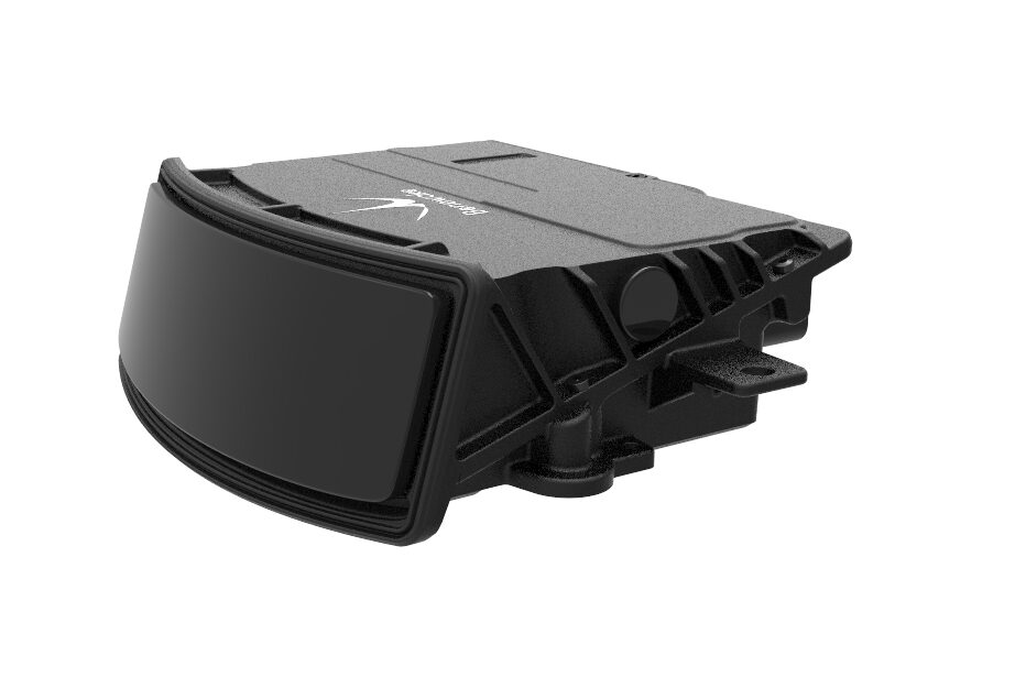
B2X2 4 Elements Infrared Motion Analog PIR Sensor for Lighting
When presence detection (not distance) is needed, this PIR motion sensor is ideal for lighting automation and security applications.
Factors That Affect IR Sensor Accuracy
1. Target Surface Properties
IR sensors using triangulation (Sharp GP2Y series) are relatively immune to target color and reflectivity because they measure position of the spot, not its intensity. However, highly specular (mirror-like) surfaces and transparent materials (glass, clear plastic) can scatter IR in unexpected ways and cause erroneous readings. Always test with the actual target material.
2. Ambient Light and Sunlight
Strong ambient IR (direct sunlight, incandescent bulbs) saturates the PSD and causes the sensor to read maximum distance even with an object close by. For outdoor use, add a physical IR-blocking shield around the sensor or switch to a modulated IR sensor (SFH4550-based designs) that uses lock-in detection to reject ambient light.
3. Temperature
The IR LED’s output intensity changes with temperature (approximately -0.5% per °C for typical GaAs LEDs). At temperatures above 40°C (common in Indian summers), the effective range may decrease by 5–10%. For high-temperature environments, perform calibration at operating temperature.
4. Power Supply Noise
IR sensor LEDs draw pulsed current, which can cause supply voltage ripple that corrupts ADC readings. Add a 100µF electrolytic capacitor (plus 10nF ceramic) across the sensor’s power supply pins, physically close to the sensor. This is especially important when the sensor is powered from the same rail as motors or other high-current loads.
5. Object Size and Angle
Very small objects (smaller than the IR beam width) may read farther than actual. Objects tilted away from perpendicular reflect less light back and read farther than actual. For best accuracy, ensure the target fills the sensor’s field of view and is perpendicular to the sensor axis.
IR vs Ultrasonic Proximity Sensors: When to Use Each
| Factor | IR Proximity (GP2Y) | Ultrasonic (HC-SR04) |
|---|---|---|
| Range | 10–150cm (model dependent) | 2cm–400cm |
| Output | Analog voltage (non-linear) | Pulse width (linear) |
| Update rate | Very fast (continuous) | ~25ms minimum cycle |
| Transparent objects | Poor (glass, water) | Excellent |
| Sunlight resistance | Poor | Excellent |
| Narrow beam | Yes (~5-10°) | Wide cone (~30°) |
| Black surfaces | Good (triangulation) | Excellent |
| Cost (India) | ₹300–600 (Sharp) | ₹50–100 (HC-SR04) |
Choose IR when: You need fast updates, small form factor, narrow field of view, or the target is soft/sound-absorbing (which fools ultrasonic sensors).
Choose ultrasonic when: You need longer range, better sunlight resistance, transparent target detection, or a budget build.
Frequently Asked Questions
Benewake AD2-S-X3 High-Performance Automotive-Grade LiDAR
When IR proximity sensor accuracy is not enough, upgrade to automotive-grade LiDAR for centimeter-accurate 3D distance sensing in demanding applications.
Conclusion
Mastering IR proximity sensor calibration and the distance vs voltage curve transforms these sensors from frustrating, imprecise devices into reliable measurement tools. The key insights: the output is an inverse power-law curve (not linear), the inverse of voltage (1/V) is approximately linear with distance, and your specific sensor unit needs individual calibration to achieve the best accuracy.
Whether you use the simple inverse linearization method or a full lookup table with interpolation depends on your accuracy requirements. For robot obstacle avoidance (±2cm is fine), the inverse formula is sufficient. For precision positioning or industrial automation, invest the extra time to build a lookup table from measured calibration data. Either way, averaging multiple ADC readings and applying a moving average filter are non-negotiable steps for stable, reliable IR distance measurement.


Add comment